Newton's Method to find roots of functions is actually super cool. Let's talk about it in the 2D (Euclidean) plane. You start with any function you want, and start with any x value. Draw a point on the function at (x, f(x)). At that point, draw a tangent line and extend it until it hits the x-axis. For that value of x where it crosses the x-axis, let's call that value x_cross. Now draw a point at (x_cross, f(x_cross)). Repeat the whole process. Eventually, assuming your function has roots, f(x_cross) will converge to zero!
I learned a bit of shell scripting and vim to write some Python code in my terminal. I had to do some math gymnastics by dusting my brain off and using the limit definition of a derivative and the point-slope form of a line. Here's my Newton's Method algorithm:
import math
max_iter = 100000 # maximum number of interations i'm allowing
usr_input = input ("Enter info for Newton's method (x_start, epsilon) : ")
x_start, eps = usr_input.split (",")
x_start = float(x_start)
eps = float(eps)
# polynomial we want the roots of
def f(x):
return (2*x*x + x + 3 - math.exp(x))
# get slope of tangent line at a point x with derivative
def slope(x):
return ((f(x+eps)-f(x))/eps)
# find x value at which line tangent to curve intersects x-axis
def get_xcross(x):
return (x - (f(x)/slope(x)))
# iterate to perform newton's method
x = x_start
y = 100 #distance from 0
cnt = 0
while abs(y) > eps:
x = get_xcross(x)
print("x is", x)
y = f(x)
cnt = cnt + 1
if cnt > max_iter:
print("oops this function seems to not have roots")
if cnt < max_iter:
print("this is the root of your function: ", x)
As an aside, putting in Python code and mixing it with HTML tags to look well-formatted is such a treat haha.
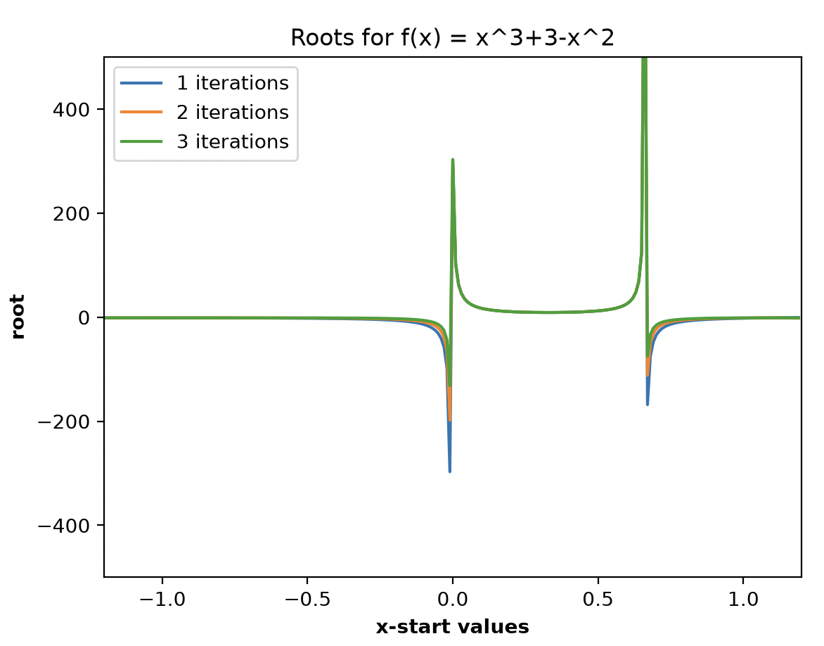
I decided to make some plots of roots that the algorithm converges to given various x starting values. I also checked out the results for varying numbers of iterations through the algorithm. Something I realized after a bit of trial-and-error is that this plot will have peaks/asymptotes where the derivative of the function is zero. That's because a tangent to my graph will be aproximately parallel to the x-axis which means that we would have a huge x_cross value where the line crosses the x-axis.
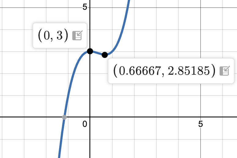
Let's inspect the function f(x) = x^3 + 3 -x^2. It's drawn on the right below. This function has one root at x = -1.17, so we should expect most of the x_start values to converge on this value. However, the derivative has two places where it is zero, so we might expect two asymptotes or spikes in this plot. See the images below!
Clearly, we can imagine drawing tangent lines to our function, and we see right at x = 0 and x = 0.67 that the tangent lines would be nearly parallel to the x-axis! Correspondingly, our root vs x_start plot has two spikes there!
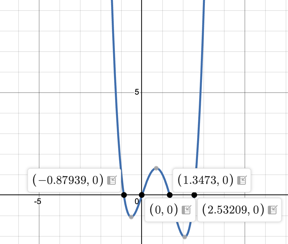
Let's look at another polynomial! f(x) = x^4-3x^3+2x+x. We see 4 healthy roots in the plot on the right, and correspondingly, our algorithm descends upon these roots like a vulture on road kill! We also see a bunch of spikes in our plot where the tangent lines to the function are approximately horizontal. I'm starting to see some self-similarity in this plot...
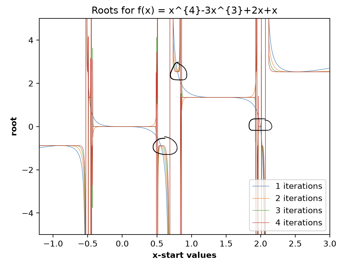
You can see that each of the four roots and the plotted attempts to find the roots have a similar shape. You can even see the algorithm have small 'hiccups' where it approaches a different root for a second! Let me show you in the range -1 < x < 0.8 below. If our x_start value is near x = -1, the algorithm should definitely find the nearby zero at x = -0.87. We see that correcty on the left- the smooth flat curve at y = -0.87. After x_start values of maybe -0.4, the algorithm starts to find the next root at x = 0. This makes sense. This is where it gets interesting...
For 0.5 < x_start < 0.65, the algorithm detects on old zero! In the plot on the right, we see our function around 0.5 < x < 0.65 is valued around 1.1 to 1.3, nowhere close to a root of -0.87. For 0.5 < x < 0.65, the nearest zeroes are 0 and 1.3. Hence, we see that trajectories starting near each other that should go to the nearest root end up getting 'attracted' to a different root!
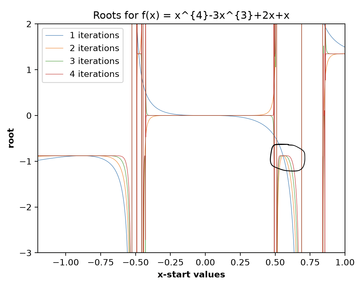
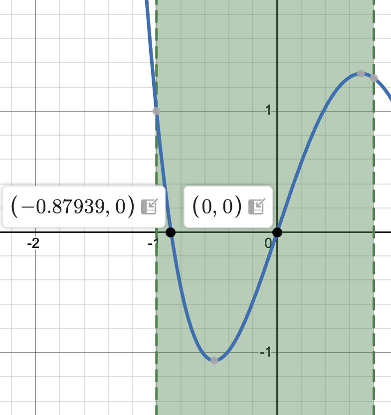
A general definition of chaos as I understand it is that a chaotic system is very sensitive to inital conditions. You can get completely different behavior of that system even when your initial conditions are extrmeley similar. In this Newton's Method algorithm, I'm seeing some hallmarks of chaos: self-similarity and attractors! Attractors are regions of phase-space where your trajectories approach it over and over, even when starting with different initial conditions. We could conceptualize the roots as an attractor that pulls trajectories towards them!
Let's look at the self-similarity! I decided to stop interpolating in my plots to turn the roots into dust instead of lines. I also decreased my step size in my algorithm:
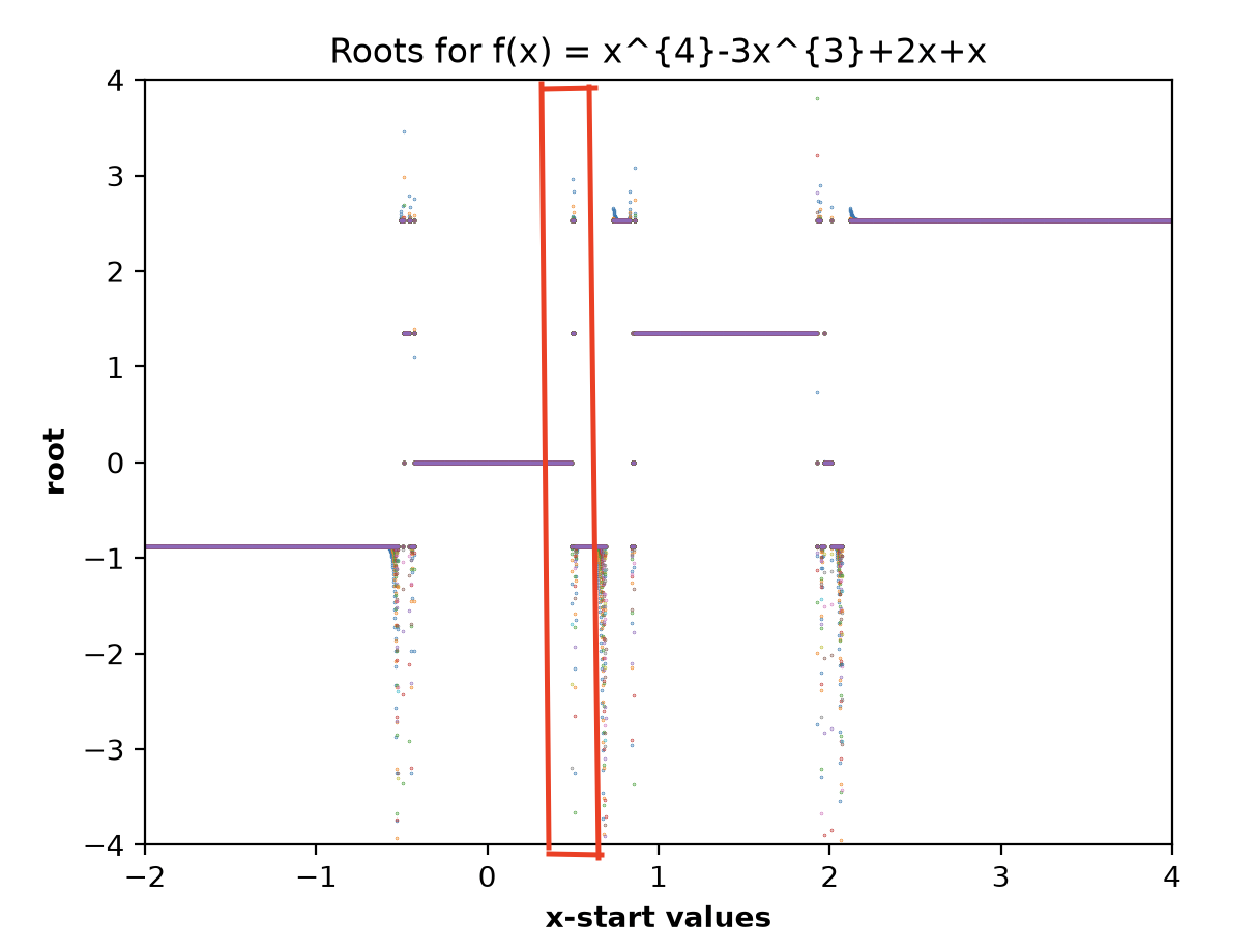
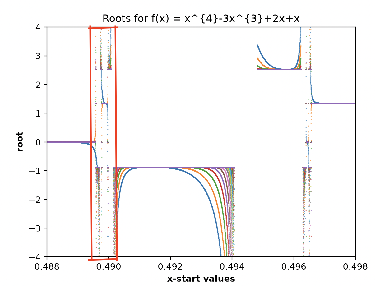
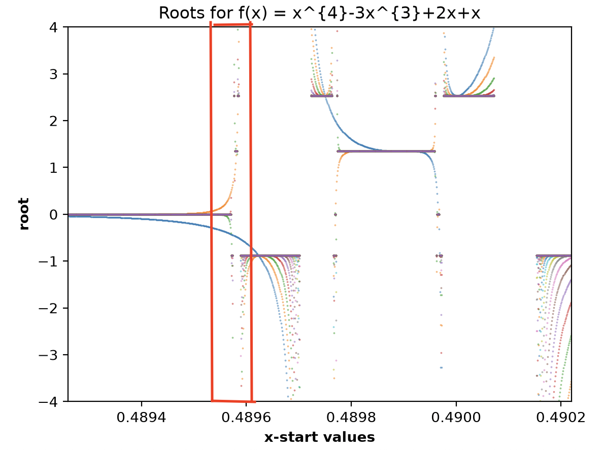
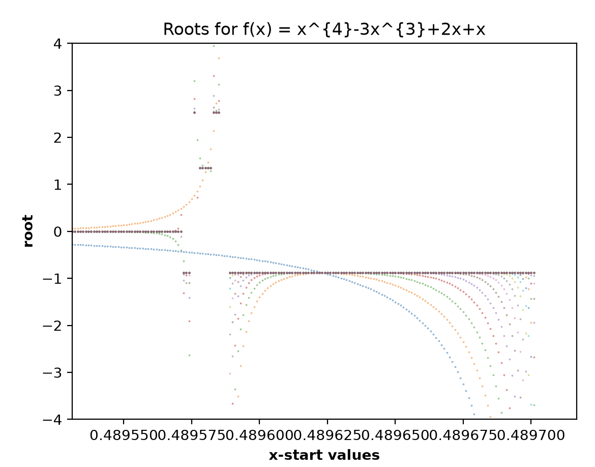
At all scales, we can see similar 'U' shapes, asymptotes made of dust, and a bunch of trajectories that get attracted back to our four roots at -0.87, 0, 1.3, and 2.5!